Categories
#rstats Data analysis ruminations Software Work

Same Developer, New Stack

I’ve been fortunate to work with and on open-source software this year. That has been the case for most of a decade: I began using R in 2014. I hit a few milestones this summer that got me thinking about my OSS journey.

I became a committer on the Apache Superset project. I’ve written previously about deploying Superset at work as the City of Ann Arbor’s data visualization platform. The codebase (Python and JavaScript) was totally new to me but I’ve been active in the community and helped update documentation.

Those contributions were sufficient to get me voted in as a committer on the project. It’s a nice recognition and vote of confidence but more importantly gives me tools to have a greater impact. And I’m taking baby steps toward learning Superset’s backend. Yesterday I made my first contribution to the codebase, fixing a small bug just in time for the next major release.

Superset has great momentum and a pleasant and involved (and growing!) community. It’s a great piece of software to use daily and I look forward to being a part of the project for the foreseeable future.

I used pyjanitor for the first time today. I had known of pyjanitor‘s existence for years but only from afar. It started off as a Python port of my janitor R package, then grew to encompass other functionality. My janitor is written for beginners, and that came full circle today as I, a true Python beginner, used pyjanitor to wrangle some data. That was satisfying, though I’m such a Python rookie that I struggled to import the dang package.

Categories
#rstats Data analysis ruminations Work

Reflections on five years of the janitor R package

One thing led to another. In early 2016, I was participating in discussions on the Twitter hashtag, a community for users of the R programming language. There, Andrew Martin and I met and realized we were both R users working in K-12 education. That chance interaction led to me attending a meeting of education data users that April in NYC.

Going through security at LaGuardia for my return flight, I chatted with Chris Haid about data science and R. Chris affirmed that I’d earned the right to call myself a “data scientist.” He also suggested that writing an R package wasn’t anything especially difficult.

My plane home that night was hours late. Fired up and with unexpected free time on my hands, I took a few little helper functions I’d written for data cleaning in R and made my initial commits in assembling them into my first software package, janitor, following Hilary Parker’s how-to guide.

That October, the janitor package was accepted to CRAN, the official public repository of R packages. I celebrated and set a goal of someday attaining 10,000 downloads.

Yesterday janitor logged its one millionth download, wildly exceeding my expectations. I thought I’d take this occasion to crunch some usage numbers and write some reflections. This post is sort of a baby book for the project, almost five years in.

By The Numbers

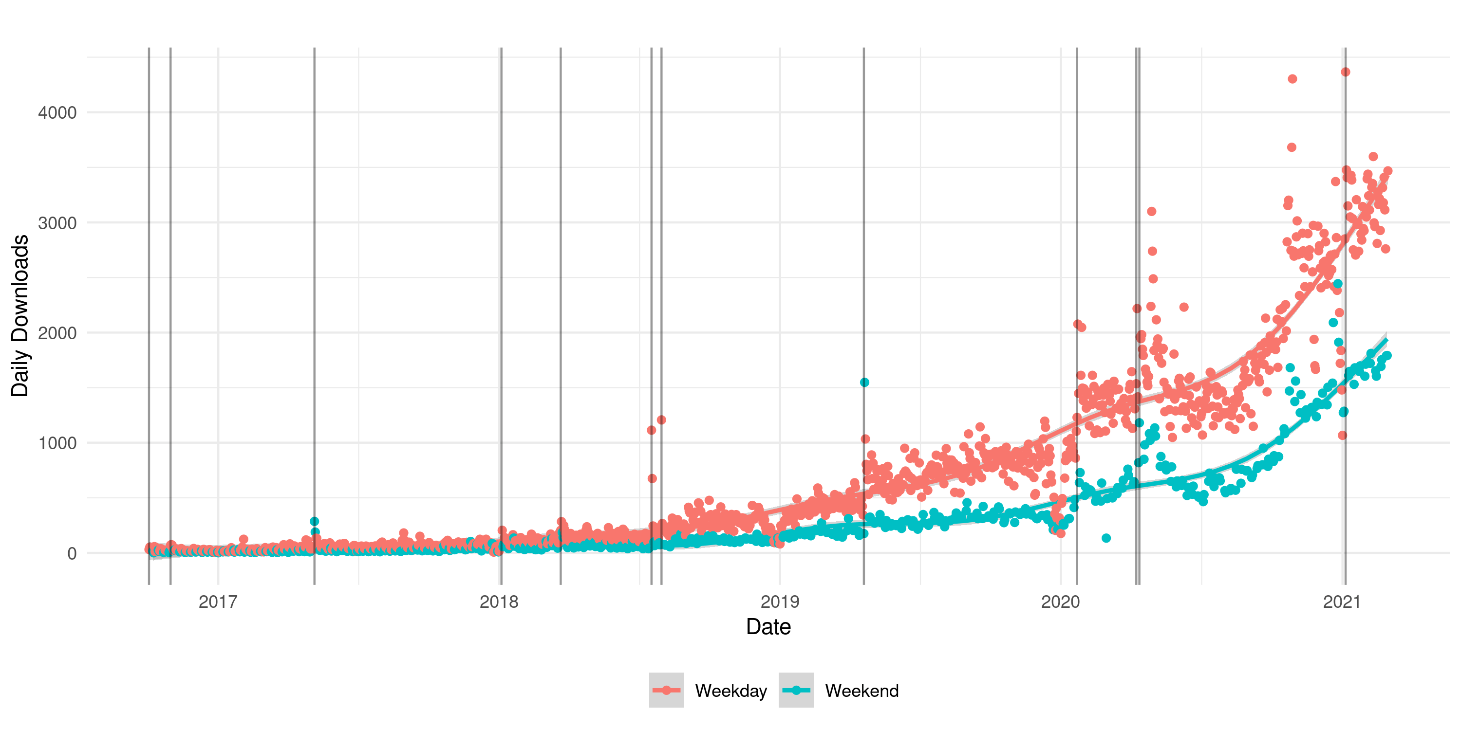
This chart shows daily downloads since the package’s first CRAN release. The upper line (red) is weekdays, the lower line (green) is weekends. Each vertical line represents a new version published on CRAN.

From the very beginning I was excited to have users, but this chart makes that exciting early usage seem miniscule. janitor’s most substantive updates were published in March 2018, April 2019, and April 2020, with it feeling more done each time, but most user adoption has occurred more recently than that. I guess I didn’t have to worry so much about breaking changes.

Another way to look at the growth is year-over-year downloads:

YearDownloadsRatio vs. Prior Year
2016-1713,284
2017-1847,3043.56x
2018-19161,4113.41x
2019-20397,3902.46x
2020-21 (~5 months)383,5956
Download counts are from the RStudio mirror, which does not represent all R user activity. That said, it’s the only available count and the standard measure of usage.
Categories
#rstats Making Work

That feeling when your first user opens an issue

You know how new businesses frame the first dollar they earn?

I wrote an R package that interfaces with the SurveyMonkey API. I worked hard on it, on and off the clock, and it has a few subtle features of which I’m quite proud. It’s paying off, as my colleagues at TNTP have been using it to fetch and analyze their survey results.

The company and I open-sourced the project, deciding that if we have already invested the work, others might as well benefit. And maybe some indirect benefits will accrue to the company as a result. I made the package repository public, advertised it in a few places, then waited. Like a new store opening its doors and waiting for that first customer.

They showed up on Friday! With the project’s first GitHub star and a bug report that was good enough for me to quickly patch the problem. Others may have already been quietly using the package, but this was the first confirmed proof of use. It’s a great feeling as an open-source developer wondering, “I built it: will they come?”

Consider this blog post to be me framing that dollar.

Categories
#rstats Data analysis Sports

Double check your work (Kaggle Women’s NCAA tournament 2019)

I’m writing about an attention-to-detail error immediately after realizing it.  It probably won’t matter, but if it ends up costing me a thousands-of-dollars prize, I’ll feel salty.  I thought I’d grouse in advance just in case.

The last few years I’ve entered Kaggle’s March Madness data science prediction contests.  I had a good handle on the women’s tournament last year, finishing in the top 10%.  But my prior data source – which I felt set me apart, as I scraped it myself – wasn’t available this year.  So, living my open-source values, I made a quick submission by forking a repo that a past winner shared on Kaggle and adding some noise.

Now, to win these contests – with a $25k prize purse – you need to make some bets, coding individual games as 1 or 0 to indicate 100% confidence that a team will win.  If you get it right, your prediction is perfect, generating no penalty (“log-loss”).  Get it completely wrong and the scoring rule generates a near-infinite penalty for the magnitude of your mistake – your entry is toast.

You can make two submissions, so I entered one with plain predictions – “vanilla” – and one where I spiced it up with a few hard-coded bets.  In my augmented Women’s tournament entry, I wagered that Michigan, Michigan State, and Buffalo would each win their first round games.  The odds of all three winning was was only about 10%, but if it happened, I thought that might be enough for me to finish in the money.

Michigan and Buffalo both won today!  And yet I found myself in the middle of the leaderboard.  I had a sinking feeling.  And indeed, Kaggle showed the same log-loss score for both entries, and I was horrified when I confirmed:

A comparison of my vanilla and spiced-up predictions
These should not be identical.

In case Michigan State wins tomorrow and this error ends up costing me a thousand bucks in early April, the commit in question will be my proof that I had a winning ticket and blew it.

Comment if you see the simple mistake that did me in:

Where is an AI code reviewer to suggest this doesn’t do what I thought it did?

As of this writing – 9 games in – I’m in 294th place out of 505 with a log-loss of 0.35880.  With the predictions above, I’d be in 15th place with a log-loss of 0.1953801, and ready to benefit further from my MSU prediction tomorrow.

The lesson is obvious: check my work!  I consider myself to be strong in that regard which makes this especially painful.  I could have looked closely at my code, sure, but the fundamental check would have been to plot the two prediction sets against each other.

That lesson stands, even if the Michigan State women fall tomorrow and render my daring entry, and this post, irrelevant.  I’m not sure I’ll make time for entering these competitions next year; this would be a sour note to end on.

Categories
#rstats Data analysis

Generating unique IDs using R

Here’s a function that generates a specified number of unique random IDs, of a certain length, in a reproducible way.

There are many reasons you might want a vector of unique random IDs.  In this case, I embed my unique IDs in SurveyMonkey links that I send via mail merge. This way I can control the emailing process, rather than having messages come from SurveyMonkey, but I can still identify the respondents.  If you are doing this for the same purpose, note that you first need to enable a custom variable in SurveyMonkey!  I call mine for simplicity.

The function

create_unique_ids <- function(n, seed_no = 1, char_len = 5){
  set.seed(seed_no)
  pool <- c(letters, LETTERS, 0:9)
  
  res <- character(n) # pre-allocating vector is much faster than growing it
  for(i in seq(n)){
    this_res <- paste0(sample(pool, char_len, replace = TRUE), collapse = "")
    while(this_res %in% res){ # if there was a duplicate, redo
      this_res <- paste0(sample(pool, char_len, replace = TRUE), collapse = "")
    }
      res[i] <- this_res
  }
  res
}

Here’s what you get:

> create_unique_ids(10)
 [1] "qxJ4m" "36ONd" "mkQxV" "ES9xW" "5nOhq" "xax1v" "DLElZ" "PXgSz" "YOWIG" "WbDTQ"

This function could get stuck in the while-loop if your N exceeds the number of unique permutations of alphanumeric strings of length char_len.  There are length(pool) ^ char_len permutations available.  Under the default value of char_len = 5, that’s 62^5 combinations or 916,132,832.  This should not be a problem for most users.

On reproducible randomization

The ability to set the randomization seed is to aid in reproducing the ID vector.  If you’re careful, and using version control, you should be able to retrace what you did even without setting seed.  There are downsides to setting the same seed each time too, for instance, if your input list gets shuffled and you’re now assigning already-used codes to different users.

No matter how you use this function, think carefully about how to record and reuse values such that IDs stay consistent over time.

Exporting results for mail merging

Here’s what this might look like in practice if you want to generate these IDs, then merge them into SurveyMonkey links and export for sending in a mail merge.  In the example below, I generate both English- and Spanish-language links.

roster$id <- create_unique_ids(nrow(roster), seed = 23)
roster$link_en <- paste0("https://www.research.net/r/YourSurveyName?a=", roster$id, "&lang=en")
roster$link_es <- paste0("https://www.research.net/r/YourSurveyName?a=", roster$id, "&lang=es")
readr::write_csv(roster, "data/clean/roster_to_mail.csv", na = "")

Note that I have created the custom variable a in SurveyMonkey, which is why I can say a= in the URL.

Categories
#rstats

Advent of Code 2017 in #rstats: Day 13

I liked the twist in the Day 13 puzzle.  Implementing a literal solution to part 1, where I had the scanners walk back and forth, was straightforward.  And Part 2 looked easy enough.  Then I peeked at how slowly my algorithm was proceeding and realized I would need to refactor.

Part 1

This function has been modified in two places for Part 2.  I added the first line in the function, using the modulo operator `%%` to trim the time down to a single back-and-forth pass.   This made the commented-out direction change line obsolete.

I worked out the `time %% ((size-1)*2)` bit by counting examples on my fingers 🙂

# Time corresponds to "depth", size = "range"

move <- function(size, time){
  time <- time %% ((size-1)*2) # added this line for part 2 to be O(n) not O(n^2)
  pos <- 1
  increment <- 1
  for(i in seq_len(time)){ # with the modulo line this could be done w/o loop
  #  if(pos == 1) { increment <- 1 } # Don't need this b/c of adding the modulo
    if(pos == size) { increment <- -1}
    pos <- pos + increment
  }
  pos
}

library(testthat)
expect_equal(move(3, 0), 1)
expect_equal(move(2, 1), 2)
expect_equal(move(4, 4), 3)
expect_equal(move(4, 6), 1)

dat <- read.csv("13_dat.txt", sep = ":", header = FALSE) %>%
  setNames(c("depth", "size"))

sum((dat$size * dat$depth)[with(dat, mapply(move, size, depth)) == 1]) # 1728

Part 2

Without the modulo line above, my loop will walk the scanner back and forth for time steps.  As the delay increases, so does the time.  The answer to this problem is a delay of approximately 4 million time units; at that point, each scanner is walked 4 million times… it’s been a long time since CS 201 but I think that makes the algorithm O(N2).  In practice, I realized I had a problem when progress slowed dramatically.

Realizing this, I eliminated the unnecessary walking.  Now, this could still be much more efficient.  Because I’m recycling code from part 1, I test all scanner depths for collisions at each iteration; a faster solution would move on to the next delay value after a single scanner collision is found.  But hey, that is a mere ~20x slowdown or so, and is still O(N).

Having started with R in 2014, I rarely feel like an old-timer.  I learned dplyr from the beginning, not tapply.  But I had that feeling here… being somewhat comfortable with `mapply` gets in the way of sitting down to learn the `map2` functions from purrr, which I suspect will be useful to know.

# Part 2

system.time({
  delay <- 0
  hits <- sum(with(dat, mapply(move, size, depth)) == 1) 
  while(
    hits != 0
  ){
    dat$depth <- dat$depth + 1
    delay <- delay + 1
    hits <- sum(with(dat, mapply(move, size, depth)) == 1)
  }
}
)

 user system elapsed 
906.512 2.804 909.319 
> delay
[1] 3946838

My runtime was about 15 minutes.

Categories
#rstats

Advent of Code 2017 in #rstats: Day 12

(Day 12 puzzle). This was my favorite day so far.  I’ve never faced my own graph problem and this was a great example for trying out the igraph package.

Big shout out to Gábor Csárdi and anyone else on the igraph team who wrote the docs.  And I mean wrote the docs!  When I google an R question, 99% of the time I land on StackOverflow.  The searches I made for Day 12 all* took me to the igraph documentation website, which answered my questions.  I don’t know of another R package or topic like that.

Their example of creating a graph was clear and was easy to adapt to the toy example on Day 12.  From there, some searching found the two functions I’d need for Day 12: neighborhood() and clusters().  Look how short my part 2 is!

Part 0: Playing with igraph

Here’s the documentation example for creating an igraph.  I played with it to confirm it would work for my needs:

library(pacman)
p_load(igraph, tidyr, dplyr)

# Toy example
relations <- data.frame(from=c("Bob", "Cecil", "Cecil", "David",
                               "David", "Esmeralda"),
                        to=c("Alice", "Bob", "Alice", "Alice", "Bob", "Alice"),
                        same.dept=c(FALSE,FALSE,TRUE,FALSE,FALSE,TRUE),
                        friendship=c(4,5,5,2,1,1), advice=c(4,5,5,4,2,3))
g <- graph_from_data_frame(relations, directed=FALSE)
neighborhood(g, 1, "Esmeralda") # 2
neighborhood(g, 2, "Esmeralda") # 5

Part 1

This was mostly wrangling the data into the igraph.  It didn’t seem to like integer names for vertices so I prepended “a”.

create_graph_from_input <- function(filename){
  filename %>%
    read.delim(header = FALSE) %>%
    separate(V1, into = c("v1", "v2"), sep = "<->") %>%
    separate_rows(v2, sep = ",") %>%
    mutate(v1 = paste0("a", str_trim(v1)),
           v2 = paste0("a", str_trim(v2))) %>%
    graph_from_data_frame(directed = FALSE)
}

get_group_size <- function(filename, grp_size, node_name){
   create_graph_from_input(filename) %>%
    neighborhood(grp_size, paste0("a", node_name)) %>%
    unlist %>%
    length()
  }
testthat::expect_equal(get_group_size("12_1_test_dat.txt", 30, "0"), 6)
get_group_size("12_1_dat.txt", 30, "0") # 239

I increased the `grp_size` parameter until my result stopped increasing.  That was at about 30 degrees of separation (it was still changing at 15).  A more permanent solution might include a loop to do this.

Part 2

All you need is igraph::clusters():

"12_1_dat.txt" %>%
  create_graph_from_input %>%
  clusters() %>%
  .$no #215

One.  Function.

Conclusion: graphs are neat, igraph is the way to analyze them.

* okay, one search took me to StackOverflow and gave me what I needed: the `clusters()` function.  Everything else came from igraph.org.

Categories
#rstats

Advent of Code 2017 in #rstats: Day 11

Once I realized that moves on a hex grid map nicely to a standard rectangular grid, this was easy.   Despite playing hours of Settlers of Catan, I’d never realized this relationship.  Maybe because nothing traverses that hex grid?

North and South move one step up or down.  The four diagonal directions move a half-step up or down and a full column laterally.  The shortest solution path will be diagonal moves to reach the desired column, then vertical moves to the right row.

It took only a minute or two to modify my part 1 function for part 2, so I present both together.

Parts 1 & 2

library(dplyr); library(testthat)

steps_needed <- function(dat){
  lat <- 0
  lon <- 0
  max_dist <- 0
  current_dist <- 0
  for(i in seq_along(dat)){
    if(dat[i] == "n"){lat <- lat + 1}
    if(dat[i] == "s"){lat <- lat - 1}
    if(dat[i] == "ne"){lat <- lat + 0.5; lon <- lon + 1}  
    if(dat[i] == "se"){lat <- lat - 0.5; lon <- lon + 1}
    if(dat[i] == "nw"){lat <- lat + 0.5; lon <- lon - 1}
    if(dat[i] == "sw"){lat <- lat - 0.5; lon <- lon - 1}
    
    current_distance <-   
      abs(lon) + # diagonal steps to move horizontally
      abs(lat) - 0.5 * abs(lon) # vertical steps, adjusted for prev diagonal moves
    
    max_dist <- max(c(max_dist), current_distance)
    current_dist <- current_distance
  }
  structure(c(current_dist, max_dist),
            names = c("Current Distance", "Maximum Distance"))
}

# Tests
expect_equal(steps_needed(c("se","sw","se","sw","sw")), 3)
expect_equal(steps_needed(c("ne", "ne", "ne")), 3)
expect_equal(steps_needed(c("ne", "ne", "sw", "sw")), 0)
expect_equal(steps_needed(c("ne", "ne", "s", "s")), 2)

# Execute
dat <- unlist(str_split(scan("11_1_dat.txt", "character"), ","))
steps_needed(dat)

# Current Distance Maximum Distance 
# 722 1551 


Categories
#rstats

Advent of Code 2017 in #rstats: Day 9

I write less deeply-nested code now that I program in R.  When writing code poorly  in other programs, I’d often use nested IF statements (hi, Excel!).  Debugging that often looked like counting my nesting depth out loud: add one for every (,  subtract one for every ).

That strategy formed the basis for my solution today.   And I was excited to do Part 2 with arithmetic, not writing new code.

Part 1

Strategy: maintain counter of open braces, decreasing for closed braces.

So `{{<a>},{<a>},{<a>},{<a>}}` = 1 2 2 2 2. Sum = 9.

library(pacman)
p_load(stringr, testthat)

# cancel the character after !
cancel_chars <- function(x){ gsub("!.", "", x) }

group_score <- function(dat){
  clean <- gsub("<.*?>", "" , dat) # non-greedy regex to remove garbage
  
  lvl <- 1 # depth of braces nesting
  counts <- rep(0, nchar(clean)) # default value for non-{ characters
  
  for(i in seq.int(nchar(counts))){
    if(str_sub(clean, i, i) == "{"){ # log the nested depth and increment counter
      counts[i] <- counts[i] + lvl
      lvl <- lvl + 1
    }
    if(str_sub(clean, i, i) == "}"){
      lvl <- lvl - 1
    }
  }
  sum(counts)
}

# Test
expect_equal(group_score("{{{}}}"), 6)
expect_equal(group_score("{{},{}}"), 5)
expect_equal(group_score("{{{},{},{{}}}}"), 16)

dat <- scan("09_1_dat.txt", "character")
group_score(cancel_chars(dat)) # 15922

Part 2

The answer is the total number of characters, minus:

  • The characters canceled by !
  • The bracketing `<>` for each garbage string
  • The valid characters remaining after removing the garbage in Part 1

To wit:

cleaned <- cancel_chars(dat)
nchar(cleaned) -
  2*str_count(string = cleaned, pattern = fixed(">")) -
  nchar(gsub("<.*?>", "" , cleaned))

# 7314


Categories
#rstats

Advent of Code 2017 in #rstats: Day 7

Today was hard, but a good challenge.  I haven’t written a recursive function since college CS – is that typical for data science / analysis work?  I don’t see much about recursion on Twitter.  Recursion feels like a separate way of thinking, and I had forgotten how.

Part 1

The first part was satisfying.  Data cleaning was quick and I thought joining the data.frame to itself to populate parent and child for each entry was a nice touch.

test <- read.delim("07_1_test_dat.txt", header = FALSE, stringsAsFactors = FALSE)

library(pacman)
p_load(tidyr, splitstackshape, readr, dplyr, stringr)

# Tidy the data
tidy_puzzle_input <- function(x){
  result <- x %>%
    separate(V1, into = c("name", "child"), sep = "->") %>%
    cSplit(., "child", ",", "long", type.convert = FALSE) %>%
    mutate(weight = parse_number(name),
           name = str_extract(name, "[A-z]+"))
  
  # Join to itself to attach parent name
  left_join(
    result,
    result %>%
      select(-weight) %>%
      rename(name = child, parent = name)
  )
}

My tidy data looked like:

        name   child weight  parent
1    jlbcwrl    <NA>     93  tzrppo
2    fzqsahw  lybovx    256  peuppj
3    fzqsahw  pdmhva    256  peuppj
4     rxivjo   mewof    206  ikdsvc
5     rxivjo  hrncqs    206  ikdsvc

Then the solution was easy:

# the bottom node will be the only one that doesn't have a parent 

test %>%
  tidy_puzzle_input %>%
  filter(is.na(parent))

read.delim("07_1_dat.txt", header = FALSE, stringsAsFactors = FALSE) %>%
  tidy_puzzle_input %>%
  filter(is.na(parent))


Part 2

This was tough going.  I got a function working for the sample input, which worked by stepping backward from the most distant children and adding their weight to their parents, then removing them and calling itself again.

But while the sample input had symmetric towers, in the bigger test data a tower could be balanced if it had two children of `4` and `2 -> 1 + 1`.  In that scenario, you can’t peel off the 4 in the same step that you peel off the 1s.  (For my own satisfaction, that false solution appears far below).

I’m proud of my eventual solution.  And besides finally getting my brain to think recursively, I learned a few things: creating a named vector with `structure()` and using `purrr::map_dbl`.

get_faulty_set <- function(dat){
  
  get_node_children <- function(node_name){
    dat$child[dat$name == node_name]
  }
  
  # recursively get the cumulative weight of a node
  get_node_weight <- function(node_name){
    if(is.na(get_node_children(node_name))[1]){
      dat$weight[dat$name == node_name][1]
    } else{
      dat$weight[dat$name == node_name][1] +
        sum(sapply(get_node_children(node_name), get_node_weight))
    }
  }
  
  # Grab parents whose children have multiple weights - the problem cascades
  faulty_parents <- dat %>%
    rowwise %>%
    mutate(total_weight = get_node_weight(name)) %>%
    group_by(parent) %>%
    summarise(num_wts = n_distinct(total_weight)) %>%
    filter(num_wts > 1) %>%
    pull(parent)
  
  # find the lowest parent where the problem occurs
  lowest_bad_parent <- dat %>%
    filter(name %in% faulty_parents) %>%
    filter(! name %in% .$parent) %>%
    slice(1) %>%
    pull(name)
  
  # Get the weights & names of that parent's children
  bad_set <- structure(
    purrr::map_dbl(get_node_children(lowest_bad_parent), get_node_weight),
    names = get_node_children(lowest_bad_parent)
  )
  bad_set
  # From here it's common sense to spot the odd node out, see how much it needs to change;
  # Then fetch its weight using get_node_weight and compute the sum
}

I finished with a cop-out: once my function returned the weights of the subtower nodes where the problem existed and their names, it wasn’t worth programming the last bit to do the weight subtraction and get my answer.  With this output:

   dkvzre awufxne   osbbt   ycbgx wdjzjlk 
   2255    2255    2255    2260    2255

I just calculated it myself using `get_node_weight(“ycbqx”)` and subtracting 5.

Appendix: Solution with Symmetric Towers

Because I feel salty that this didn’t work.

find_unbalanced_tower <- function(x){
  lowest_children <- x %>%
    filter(is.na(child)) %>%
    distinct(.keep_all = TRUE)
  
  res <- lowest_children %>%
    group_by(parent) %>%
    summarise(uniques = n_distinct(weight),
              total_wt = sum(weight))
  
  # check for completion and return result if done
  if(!all(res$uniques == 1)){
    problem_parent <- res$parent[res$uniques == 2]
    print(paste("Problem parent is: ", problem_parent))
    lowest_children %>%
      filter(parent == problem_parent) %>%
      group_by(name) %>%
      slice(1)
    
  } else {
    # Then add their weight to parent weight, remove them, update parents to have no children
    x <- x %>%
      mutate(child = ifelse(child %in% lowest_children$name, NA, child)) %>%
      filter(!name %in% lowest_children$name) %>%
      rowwise() %>%
      mutate(weight = weight + sum(res$total_wt[res$parent == name])) %>%
      ungroup() %>%
      distinct(.keep_all = TRUE)
    
    find_unbalanced_tower(x)
  }
}

my_input %>%
  tidy_puzzle_input %>%
  find_unbalanced_tower()